Tensorboard on gcloud
Word Vectors are an amazing creation from Tomas Mikolov. If you are into deep learning and NLP, you likely are familiar with them. One amazing features of word vectors is they can be interpreted using nearby words with cosine or euclidean distance metrics. For example, consider this infamous vector linear combination:
$vec(‘king’) - vec(‘man’) + vec(‘female’) = vec(‘queen’)$
For convenience, these vectors are put together as a matrix and are called word embeddings. This embedding matrix row ID is mapped to a list of words that can be thought of as a vocabulary of the whole text you are working with. Each row represents a word, and columns are features (it can be anything, 200 in my case). These features need to be learned using methods suggested in the landmark paper Efficient Estimation of Word Representations in Vector Space. I usually prefer skip-gram, but it depends on the task at hand. Once learned, they can be viewed in a lower dimensional space for visual interpretation.
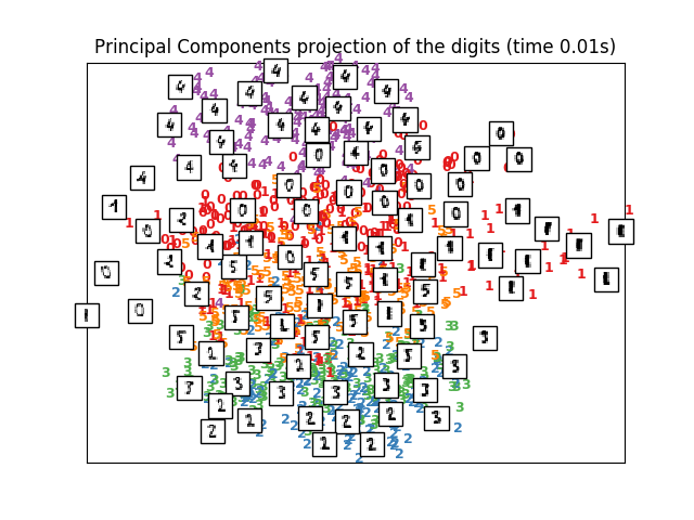
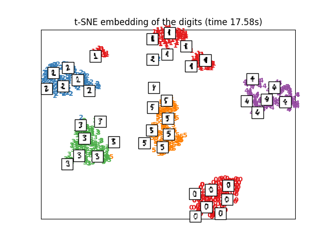
There are many methods for representing high dimensional vectors in lower dimensions for viewing and interpretation. A well-known method for converting from higher to lower dimensions is PCA and t-SNE. SKlearn has amazing APIs for them. The following pictures are taken from sklearn documentation. t-SNE is amazing, but its important to know how to use it (you can learn at distill-pub).
 |
 |
Ultimately, Google’s tensorboard is the best I have come across so far for visualizing word embeddings in 3d. While taking a CS20si course online, the instructors notes/slides/code showed how to use it, and since then I have always viewed embeddings using tensorboard.
After a long period of learning, I joined my first kaggle competition (also MLND capstone) called Personalized Medicine: Redefining Cancer Treatment. I do not have any background in medicine and I don’t think anyone wants to team up with me since this is my first kaggle ride :) However, I do have some friends in medicine and they generously looked into the word vectors and assessed their quality.
I came across free gcloud instances while completing an assignment for the most awaited course of 2017: CS231n. I hosted the embeddings there for my friends to view and assess the quality of the embeddings. This system has worked well so far.
I do have to mention tensorflow project projector.tensorflow, on which one can load the meta files to gist and host the embeddings just as I intend describe in this post. However, I noticed tensorflow project handles 5,000-10,000 words well, but with 50,000 to 100,000 words it frequently crashes on the browser. The most anyone can view and process on tensorboard is 100000 words.
Setting up gcloud instance:
CS231n has a great tutorial for painlessly setting up a Google cloud instance with ubuntu. I made a copy of the pdf just in case they take the link down. By the end of cs231n setup tutorial, you will have an instance running in the gcloud by the default name “instance-1”. I strongly suggest getting the gcloud-console-app, which makes it easy to stop and start the instance since the $$$ meter is ON once the instance starts :) I usually ask my friends when they can view the embeddings and keep the instance alive during that period of time. The pdf will instruct you to setup jupyter notebook and some other tools for completing the assignments. I didn’t follow any of those instructions since my task was not to complete their assignments. Some additional settings to tweak while setting up the tensorboard server include:
-
Install gcloud compute tools for command line tools. I use ubunutu 16.04 Server for my projects, so my remote and local machines are both ubuntu. Follow the official documentation and make sure to test the command line access to your instance. I have my default instance name as “instance-1”. Zone information is important.
-
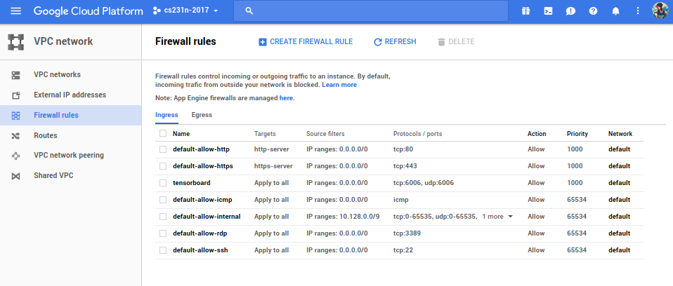
Tensorboard runs in the default port 6006. I didn’t change it. You have to set up firewall rules for outside words to communicate through the port. Go to the Google cloud console dashboard, then select VPC network on the sidebar and select Firewall rules. Add a rule as mentioned below.
-
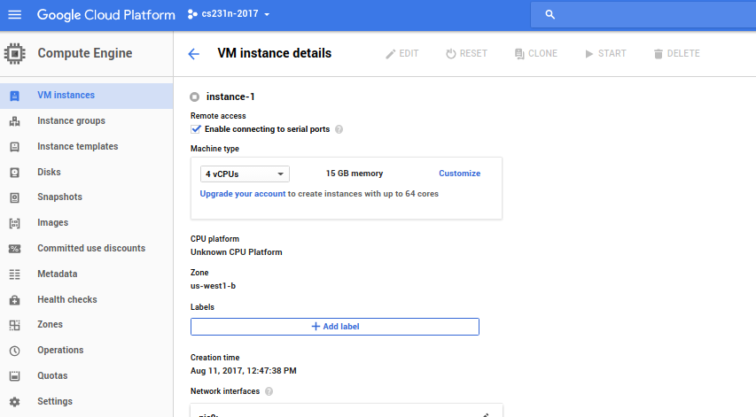
Now, in the dashboard, click Compute Engine in the side bar and it will take you to the page VM instances. Next, click on the instance name, which will take you to the page VM instance details. Click on EDIT on the top bar.
-
On this edit page, click the check-box that says Enable connecting to serial ports. This will enable you to look at the instance logs using serial connection, which will aid debugging startup scripts and such.
-
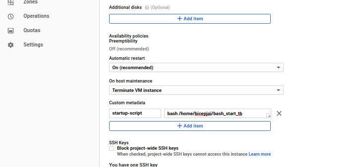
Also, under the Custom metadata section, add a key-value item (don’t use quotes there)
- startup-script as key
- bash /home/< username >/bash_start_tb as value
-
Viewing embedding on Tensorboard:
Tensorboard is used to display summaries during training on losses, display the computational graph, and, in our case, display embeddings and perform t-SNE on them. For the tensorboard to show these details, you must provide embedding details. The embedding matrix and vocabulary are formed in the same order as the embedding matrix rows. The following code generates the meta files that are required for the tensorboard to process and display.
The following processing is done on the local machine. Lets say we have the vocab list and the embedding matrix and we intend to display 100,000 words. I usually process and save them for this usage.
   vocab_words = np.load("vocab_words.npy") # vocab_size > 100000
   word_vectors = np.load("word_vectors.npy") # vector of dimensions (vocab_size, feature_size of vector dimension)
   tb_vocab_size = 10000
Tensorboard requires the metafile for vocabulary to be in tsv format. Lets create them. The necessary contents are placed in a directory name gcloud_tb
   import csv
   local_tb_dir="./gcloud_tb/"
   with open(local_tb_dir+"/vocab.tsv", "wb") as fp:
      wr = csv.writer(fp, delimiter='\n')
      wr.writerow(vocab_words[:tb_vocab_size])
Remote machine path /home/< username >/projects/tb_visual is where all the tensorboard metafiles are residing or will be transferred to. The following code snippet creates tensorboard metafiles inside the gcloud_tb directory. The metadata_path variable holds the path that is valid in a remote machine, which we will set up or update when necessary.
   visualize_this_embedding = word_vectors[:tb_vocab_size]
   print visualize_this_embedding.shape # should be of shape (tb_vocab_size, feature_size of vector dimension)
   metadata_path = "/home/<username>/projects/tb_visual/vocab.tsv"
   visualize_embeddings_in_tensorboard(visualize_this_embedding, metadata_path, local_tb_dir)
visualize_this_embedding = word_vectors[:tb_vocab_size]
print visualize_this_embedding.shape # should be of shape (tb_vocab_size, feature_size of vector dimension)
metadata_path = "/home/<username>/projects/tb_visual/vocab.tsv"
visualize_embeddings_in_tensorboard(visualize_this_embedding, metadata_path, local_tb_dir)Lets look at the function visualize_embeddings_in_tensorboard,
   import tensorflow as tf
   def visualize_embeddings_in_tensorboard(final_embedding_matrix, metadata_path, dir_path):
       """
       view the tensors in tensorboard with PCA/TSNE
       final_embedding_matrix: embedding vector
       metadata_path: path to the vocabulary indexing the final_embedding_matrix
       """
       with tf.Session() as sess:
           embedding_var = tf.Variable(final_embedding_matrix, name='embedding')
           sess.run(embedding_var.initializer)

           config = projector.ProjectorConfig()

           # add embedding to the config file
           embedding = config.embeddings.add()
           embedding.tensor_name = embedding_var.name

           # link this tensor to its metadata file, in this case the first 500 words of vocab
           embedding.metadata_path = metadata_path

           visual_summary_writer = tf.summary.FileWriter(dir_path)

           # saves a configuration file that TensorBoard will read during startup.
           projector.visualize_embeddings(visual_summary_writer, config)

           saver_embed = tf.train.Saver([embedding_var])
           saver_embed.save(sess, dir_path+'/visual_embed.ckpt', 1)

           visual_summary_writer.close()
Now all the required files will be in the directory gcloud_tb, but one file checkpoint will contain a key value pair referring to paths in the local machine where the above code is run. We have to update them to reflect the paths being setup in the remote machine (which will be discussed later)
   checkpoint_txt = "model_checkpoint_path: \"/home/<username>/projects/tb_visual/visual_embed.ckpt-1\"\n\
   all_model_checkpoint_paths: \"/home/<username>/projects/tb_visual/visual_embed.ckpt-1\""
   with open(local_tb_dir+"/checkpoint","w") as f:
       f.seek(0)
       f.truncate()
       f.write(checkpoint_txt)
Setting up remote and local scripts:
I have some handy bash aliases for executing command line arguments. Put these in your local machine bash profile file and source them.
   #serve tensorboard on google computer
   alias gclogin="gcloud compute ssh --zone=us-west1-b instance-1"
   alias gcserial="gcloud compute connect-to-serial-port instance-1"
   alias gc_tb_clean="gcloud compute ssh <username>@instance-1 --command 'rm -rf ~/projects/tb_visual/*'"
   function gc_tb_scp () {
     gcloud compute scp $@ <username>@instance-1:~/projects/tb_visual/ ;
   }
   alias gc_tb_update="gc_tb_clean && gc_tb_scp"
alias gc_tb_restart="gcloud compute ssh <username>@instance-1 --command 'bash /home/<username>/bash_restart_tb &'"-
Start the instance and on a terminal immediately execute
gclogin. Wait while it logs in. This needs to be set up before we execute any more commands on the terminal for gcloud instance. -
After this, on a new terminal, execute
gcserial. This will open a serial connection that will be live until the instance is shutdown. Any startup issues can be debugged here. -
Now, use
gcloginto log into the instance -
Install anaconda2. Make an environment named
tensorflow. Then install tensorflow and tensorboard. This should be fairly easy. Usually, I prefer creating a software folder namedprograms. -
Create
bash_start_tbbash script. This is the one we put in the gcloud Custom metadata section. This will be called during start up and you can use the serial connection terminal window started above to debug any issues.
   #! /bin/bash
   export PATH="/home/<username>/programs/anaconda2/bin:$PATH"
   source /home/<username>/programs/anaconda2/envs/tensorboard/bin/activate tensorboard
/home/<username>/programs/anaconda2/bin/tensorboard --logdir=/home/<username>/projects/tb_visual --port=6006 &- Create another script called
bash_restart_tb. This can be used to restart tensorboard if there are issues or after we have new data uploaded for rendering.
   #! /bin/bash
   for pid in $(ps -ef | grep "tensorboard.py --logdir" | awk '{print $2}'); do sudo kill -9 $pid; done;
   bash /home/<username>/bash_start_tb
Update Tensorboard at will:
Now the instance is set up. You can generate tensorboard meta files at will using the above procedure on the local machine, say in folder ~/gcloud_tb_stuff. The aliases for the commands and the bash scripts on the remote machine expects the tensorboard files to be located at ~/projects/tb_visual.
-
To clean the remote instance tensorboard folder and update the new set of meta files created, we can use the command
gc_tb_update <local_folder_containing_tb_meta_files>/*. -
Issuing
gc_tb_restartwill restart the tensorboard remotely, and hence new data will be rendered. -
When trying the view the tensorboard on any browser, use http and not https, which is default. http://< instance-ip >:6006/
That’s it! Just don’t forget to shutdown your instances after usage :) Show tensorboard to you friends whose field you are trying to disrupt with machine learning and get them to experience the following equality.
MIND = BLOWN
Let me know if you have any questions ! and please do correct me if somethings are off !