Deep (Survey) Text Classification Part 1
Natural Language Processing (NLP) tasks, such as part-of-speech tagging, chunking, named entity recognition, and text classification, have been subject to a tremendous amount of research over the last few decades. Text Classification has been the most competed NLP task in Kaggle and other similar competitions. Count based models are being phased out (are they ?) , while new deep learning models are emerging almost every week (may be every month). This project surveys a range of neural based models for text classification task. Models selected, based on CNN and RNN, are explained with code (keras with tensorflow) and block diagrams from papers. The models are evaluated using one active kaggle competition medical datasets msk-redefining-cancer-treatment. All of them will be technical overview and for details please refer paper. This post assumes reader has good background in NN and CNN. Following models are explored.
- CNN for Sentence Classification
- DCNN for Modelling Sentences
- VDNN for Text Classification
- Multi Channel Variable size CNN
- Multi Group Norm Constraint CNN
- RACNN Neural Networks for Text Classification
Let dive right in to it.
CNN for Sentence Classification
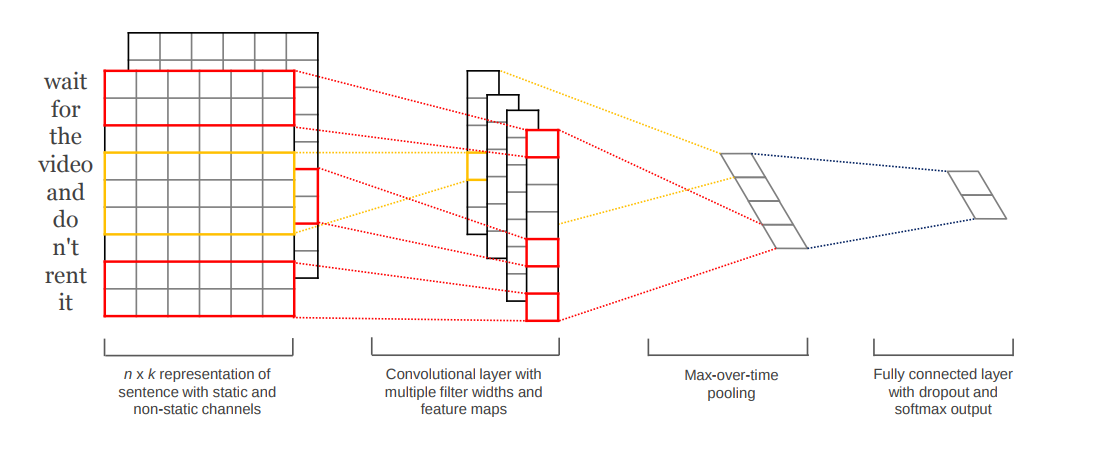
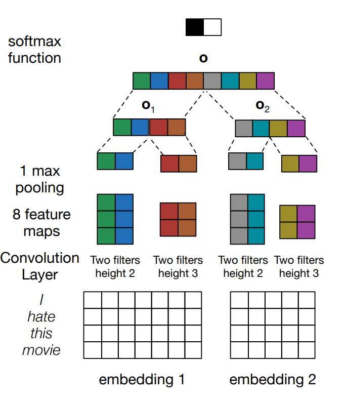
Yoon et al (2014) proposed CNN models in addition to pre-trained word vectors, which achieved excellent results on multiple benchmarks. The model architecture as shown in the figure below maintains multiple channels of input such as different types of pre-trained vectors or vectors that are kept static during training. Then they are convolved with different kernels/filters to create sets of features that are then max pooled. These features form a penultimate layer and are passed to a fully connected softmax layer whose output is the probability distribution over labels.
The paper presents several variants of the model:
- CNN-rand (a baseline model with randomly initialized word vectors)
- CNN-static (model with pre-trained word vectors)
- CNN-non-static (same as above but pre-trained fine tuned)
- CNN-multichannel (model with 2 sets of word vectors)
Lets look at the keras code for the model
text_seq_input = Input(shape=(MAX_TEXT_LEN,), dtype='int32')
text_embedding = Embedding(vocab_size, WORD_EMB_SIZE, input_length=MAX_TEXT_LEN,
                            weights=[trained_embeddings], trainable=True)(text_seq_input)

filter_sizes = [3,4,5]
convs = []
for filter_size in filter_sizes:
    l_conv = Conv1D(filters=128, kernel_size=filter_size, padding='same', activation='relu')(text_embedding)
    l_pool = MaxPool1D(filter_size)(l_conv)
    convs.append(l_pool)

l_merge = Concatenate(axis=1)(convs)
l_cov1= Conv1D(128, 5, activation='relu')(l_merge)
# since the text is too long we are maxpooling over 100
# and not GlobalMaxPool1D
l_pool1 = MaxPool1D(100)(l_cov1)
l_flat = Flatten()(l_pool1)
l_dense = Dense(128, activation='relu')(l_flat)
l_out = Dense(9, activation='softmax')(l_dense)
model_1 = Model(inputs=[text_seq_input], outputs=l_out)
Keras model summary and complete code for CNN-non static can be found here
DCNN for Modeling Sentences
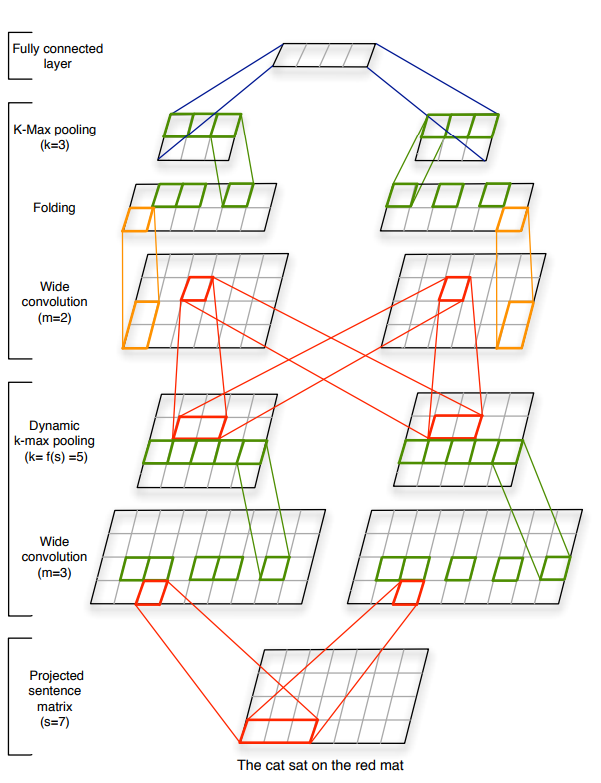
Kalchbrenner et al (2014) presented Dynamic Convolutional Neural Network for semantic modeling of sentences. This model handles sentences of varying length and uses dynamic k-max pooling over linear sequences. This helps the model induce a feature graph that is capable of capturing short and long range relations. K-max pooling, different from local max pooling, outputs k-max values from the necessary dimension of the previous convolutional layer. For smooth extraction of higher order features, this paper introduces Dynamic k-max pooling where the k in the k-max pooling operation is a function of the length of the input sentences.
\[k = max ( k_{top}, \lfloor \frac{L − l}{L} . s \rfloor )\]where $l$ is the number of convolutional layer to which pooling is applied, $L$ is total number of convolutional layers, $k_{top}$ is the fixed pooling parameter of the top most convolutional layer. The model also has a folding layer which sums over every two rows in the feature-map component wise. This folding operation is valid since feature detectors in different rows are independent before the fully connected layers.
Wide convolutions are preferred for the model instead of narrow convolutions. This is achieved in the code using appropriate zero padding.
This network model’s performance is related to its ability to capture the word and n-gram order in the sentences and to tell the relative position of the most relevant n-grams. The model also has the advantage of inducing a connected, directed acyclic graph with weighted edges and a root node as shown below.
Folding and K-max pooling layers are not readily available and have to be created using keras functional apis.
Lets look at the keras code for the model (simple right, keras rocks)
model_1 = Sequential([
    Embedding(vocab_size, WORD_EMB_SIZE, weights=[trained_embeddings],
              input_length=MAX_TEXT_LEN,trainable=True),
    ZeroPadding1D((49,49)),
    Conv1D(64, 50, padding="same"),
    KMaxPooling(k=5, axis=1),
    Activation("relu"),
    ZeroPadding1D((24,24)),
    Conv1D(64, 25, padding="same"),
    Folding(),
    KMaxPooling(k=5, axis=1),
    Activation("relu"),
    Flatten(),
    Dense(9, activation="softmax")
])
Refer code for KMaxPooling and Folding. Keras model summary and code for DCNN can be found here.
Medical CNN by Hughes et al (2017) is very similar model. Refer here for code
VDNN for Text Classification
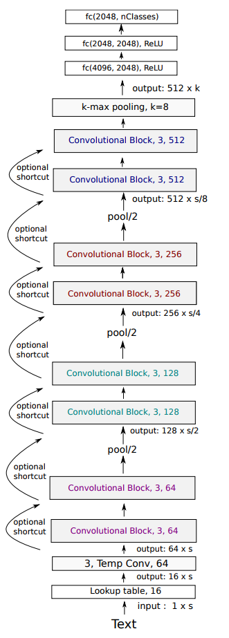
Conneau et al (2016) presented Very Deep CNN, which operates directly at the character level. This model also shows that deeper models perform better and are able to learn hierarchical representations of whole sentences.
The overall architecture of the model contains multiple sequential convolutional blocks. The two design rules followed are:
- For the same output temporal resolution, the layers have the same number of feature maps
- When the temporal resolution is halved, the number of feature maps are doubled. This helps reduce memory footprint of the model.
The model contains three pooling operations that halve the resolution each time resulting in three levels of 128, 256, 512 feature maps. There is an optional shortcut connection between the convolutional blocks that can be used, but since the results show no improvement in evaluation, that component was dropped in this project.
Each convolutional block is a sequence of convolutional layers, each followed by batch normalization layer and relu activation. The down sampling of the temporal resolution between the conv layers ( $K_i$ and $K_{i+1}$) in the block are subjected to multiple options:
- The first conv layer $K_{i+1}$ has stride 2
- $K_i$ is followed by k-max pooling layer where k is such that resolution is halved
- $K_i$ is followed by max pooling layer with kernel size 3 and stride 2
Characters used in character vectors for all the models in this paper are $abcdefghijklmnopqrstuvwxyz0123456789-,;.!?:’"/| #$%ˆ&*˜‘+=<>()[]{}$
This model is super deep, still the code is simple
Lets look at the keras code for the model.
model_1 = Sequential([
    Embedding(global_utils.CHAR_ALPHABETS_LEN, CHAR_EMB_SIZE, weights=[char_embeddings],
               input_length=MAX_CHAR_IN_SENT_LEN, trainable=True),
    Conv1D(64, 3, padding="valid")
])

# 4 pairs of convolution blocks followed by pooling
for filter_size in [64, 128, 256, 512]:

    # each iteration is a convolution block
    for cb_i in [0,1]:
        model_1.add(Conv1D(filter_size, 3, padding="same"))
        model_1.add(BatchNormalization())
        model_1.add(Activation("relu"))
        model_1.add(Conv1D(filter_size, 3, padding="same")),
        model_1.add(BatchNormalization())
        model_1.add(Activation("relu"))

    model_1.add(MaxPooling1D(pool_size=2, strides=3))

# model.add(KMaxPooling(k=2))
model_1.add(Flatten())
model_1.add(Dense(4096, activation="relu"))
model_1.add(Dense(2048, activation="relu"))
model_1.add(Dense(2048, activation="relu"))
model_1.add(Dense(9, activation="softmax"))
Keras model summary and code for VDNN can be found here.
Multi Channel Variable size CNN
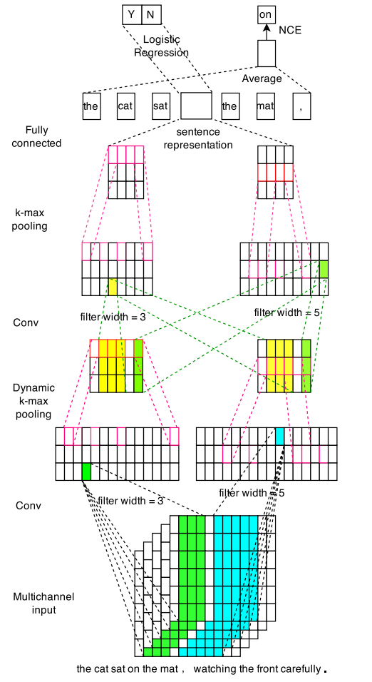
Yin et al (2016) propose MV-CNN, which combines diverse versions of pre-trained word embeddings and extract features from multi-granular phrases with variable-size convolutions. Using multiple embeddings of the same dimension from different sets of word vectors should contain more information that can be leveraged during training.
The paper describes maintaining three dimensional embedding matrices with each channel representing a different set of text embeddings. This multi-channel initialization might help unknown words across different embeddings. Frequent words can have multiple representations and rare words (partially known words) can be made up with other words. The model then has two sets of convolutional layers and dynamic k-max pooling layers followed by a fully connected layer with softmax (or logistic) as the last layer.
The paper describes two tricks for model enhancement. One is called mutual learning, which is implemented in this project. The same vocabulary is maintained across the channels and they help each other tune parameters while training. The other trick is to enhance the embeddings with pretraining just like a skip-gram model or autoencoder using noise-contrastive estimation.
Different sets of embeddings used for this model comes from glove, word2vec and custom trained vectors (data taken from the train and test corpus for unsupervised training for word vectors using fast text tool).
Lets look at the keras code for the model.
text_seq_input = Input(shape=(MAX_SENT_LEN,), dtype='int32')
text_embedding1 = Embedding(vocab_size, WORD_EMB_SIZE, input_length=MAX_SENT_LEN,
                            weights=[trained_embeddings1], trainable=True)(text_seq_input)
text_embedding2 = Embedding(vocab_size, WORD_EMB_SIZE, input_length=MAX_SENT_LEN,
                            weights=[trained_embeddings2], trainable=True)(text_seq_input)

k_top = 4
filter_sizes = [3,5]

layer_1 = []
for text_embedding in [text_embedding1, text_embedding2]:
    conv_pools = []
    for filter_size in filter_sizes:
        l_zero = ZeroPadding1D((filter_size-1,filter_size-1))(text_embedding)
        l_conv = Conv1D(filters=128, kernel_size=filter_size, padding='same', activation='tanh')(l_zero)
        l_pool = KMaxPooling(k=30, axis=1)(l_conv)
        conv_pools.append((filter_size,l_pool))
    layer_1.append(conv_pools)

last_layer = []
for layer in layer_1: # no of embeddings used
    for (filter_size, input_feature_maps) in layer:
        l_zero = ZeroPadding1D((filter_size-1,filter_size-1))(input_feature_maps)
        l_conv = Conv1D(filters=128, kernel_size=filter_size, padding='same', activation='tanh')(l_zero)
        l_pool = KMaxPooling(k=k_top, axis=1)(l_conv)
        last_layer.append(l_pool)

l_merge = Concatenate(axis=1)(last_layer)
l_flat = Flatten()(l_merge)
l_dense = Dense(128, activation='relu')(l_flat)
l_out = Dense(9, activation='softmax')(l_dense)
model_1 = Model(inputs=[text_seq_input], outputs=l_out)
Keras model summary and complete code for MVCNN can be found here.
Multi Group Norm Constraint CNN
Ye Zhang et al (2016) proposed MG(NC)-CNN and captures multiple features from multiple sets of embeddings that are concatenated at the penultimate layer. MG(NC)-CNN is very similar to MV-CNN but addresses some drawbacks, such as model complexity and requirements for the dimension of embeddings to be the same.
MG-CNN uses off the shelf embeddings and treats them as distinct groups for performing convolutions following up with max-pooling layer. Because of its simplicity, the model requires training time in the order of hours. MGNC-CNN differs in the regularization strategy. It imposes grouped regularization constraints, independently regularizing the sub-components from each separate group (embeddings). Intuitively, this captures discriminative properties of the text by penalizing weight estimates for features derived from less discriminative embeddings. Different sets of trained embeddings and l2-norm regularizer will be used in the implementation.
Lets look at the keras code
text_seq_input = Input(shape=(MAX_SENT_LEN,), dtype='int32')
text_embedding1 = Embedding(vocab_size, WORD_EMB_SIZE1, input_length=MAX_SENT_LEN,
                            weights=[trained_embeddings1], trainable=True)(text_seq_input)
text_embedding2 = Embedding(vocab_size, WORD_EMB_SIZE2, input_length=MAX_SENT_LEN,
                            weights=[trained_embeddings2], trainable=True)(text_seq_input)
text_embedding3 = Embedding(vocab_size, WORD_EMB_SIZE3, input_length=MAX_SENT_LEN,
                            weights=[trained_embeddings3], trainable=True)(text_seq_input)

k_top = 4
filter_sizes = [3,5]

conv_pools = []
for text_embedding in [text_embedding1, text_embedding2, text_embedding3]:
    for filter_size in filter_sizes:
        l_zero = ZeroPadding1D((filter_size-1,filter_size-1))(text_embedding)
        l_conv = Conv1D(filters=16, kernel_size=filter_size, padding='same', activation='tanh')(l_zero)
        l_pool = GlobalMaxPool1D()(l_conv)
        conv_pools.append(l_pool)

l_merge = Concatenate(axis=1)(conv_pools)
l_dense = Dense(128, activation='relu', kernel_regularizer=l2(0.01))(l_merge)
l_out = Dense(9, activation='softmax')(l_dense)
model_1 = Model(inputs=[text_seq_input], outputs=l_out)
Keras model summary and code for MGCNN can be found here.
RACNN Neural Networks for Text Classification
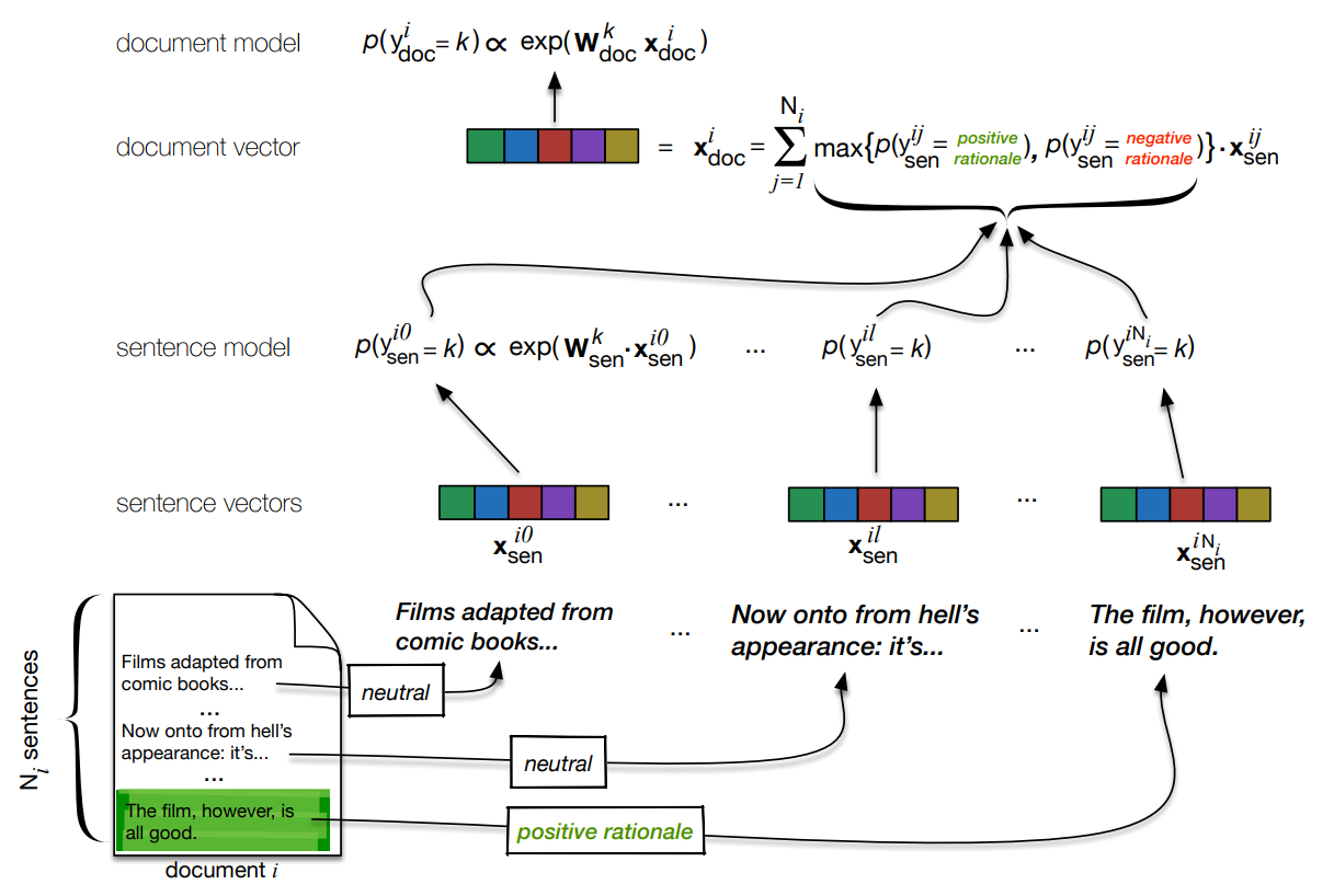
Ye Zhang et al presents RA-CNN model that jointly exploits labels on documents and their constituent sentences. The model tries to estimate the probability that a given sentence is rationales and then scale the contribution of each sentence to aggregate a document representation in proportion to the estimates. Rationales are sentences that directly support document classification.
To make the understanding of RA-CNN simpler, authors explain Doc-CNN model. In this model, a CNN model is applied over each sentence in a document and then all the generated sentence level vectors are added to form a document vector. As before, we add a softmax layer to perform document classification. Regularization is applied to both the document and sentence level vector output.
RA-CNN model is same as Doc-CNN but document vector is created as weighted sum of its constituent sentence. There are 2 stages in training this architecture, sentence level training and document level training.
For the former stage, each sentence is provided with 3 classes positive rationales, negative rationales and neutral rationales. Then with a softmax layer parametrized with its own weights (will contain 3 vectors, one for each class) over the sentences, we fit this sub-model to maximize the probabilities of the sentences being one of the rationales class. This would provide the conditional probability estimates regarding whether the sentence is a positive or negative rationale.
For the document level training, the document vector is estimated using the weighted sum of the constituent sentence vectors. The weights are set to the estimated probabilities that corresponding sentences are rationales in the most likely direction. The probabilities considered for the weights are maximum of 2 classes positive and negative rationale (neutral class is omitted). The intuition is that sentences likely to be rationales will have greater influence on the resultant document vector. The final document vector is used to perform classification on the document labels. When performing document level training, we freeze the sentence weights $W_{sen}$ and initialize the embeddings and other conv layer parameters tuned during sentence level training.
Lets look at the keras code for RA-CNN
doc_input = Input(shape=(MAX_DOC_LEN,MAX_SENT_LEN,), dtype="int32")
reshape_1d = Reshape([MAX_DOC_LEN * MAX_SENT_LEN])(doc_input)
doc_embedding_1d = Embedding(vocab_size, WORD_EMB_SIZE, weights=[trained_embeddings], trainable=True)(reshape_1d)
# data_format='channels_first' for conv2d
doc_embedding = Reshape([1, MAX_DOC_LEN, MAX_SENT_LEN * WORD_EMB_SIZE])(doc_embedding_1d)

sent_convs_in_doc = []
ngram_filters = [2,3]
n_filters = 32 # nof features
final_doc_dims = len(ngram_filters) * n_filters

# using Conv2D instead of Conv1D since we need to deal with sentences and not the whole document
# All Input shape: 4D tensor with shape: (samples, channels, rows, cols) if data_format='channels_first'
for n_gram in ngram_filters:
    l_conv = Conv2D(filters = n_filters,
                    kernel_size = (1, n_gram * WORD_EMB_SIZE), # n_gram words
                    strides = (1, WORD_EMB_SIZE), # one word
                    data_format='channels_first',
                    activation="relu")(doc_embedding)
    # this output (n_filters x max_doc_len x 1)
    l_pool = MaxPooling2D(pool_size=(1, (MAX_SENT_LEN - n_gram + 1)),
                       data_format='channels_first')(l_conv)

    # flip around, to get (1 x DOC_SEQ_LEN x n_filters)
    permuted = Permute((2,1,3)) (l_pool)

    # drop extra dimension
    reshaped = Reshape((MAX_DOC_LEN, n_filters))(permuted)
    sent_convs_in_doc.append(reshaped)

sent_vectors = concatenate(sent_convs_in_doc)
# do we need dropout here, we might lose information
# l_dropout = Dropout(0.5)(l_concat)

sentence_softmax = Dense(9, activation='softmax', kernel_regularizer=l2(0.01), name="sentence_prediction")
doc_sent_output_layer = TimeDistributed(sentence_softmax, name="sentence_predictions")(sent_vectors)

# weights are set to the estimated probabilities that
# corresponding sentences are rationales in the most likely direction
sum_weighting_probs = Lambda(lambda x: K.max(x, axis=1))

# distributing over sentences in the document
sent_weights = TimeDistributed(sum_weighting_probs)(doc_sent_output_layer)

# reshaping the weights to perform matrix dot product
reshaped_sent_weights = Reshape((1, MAX_DOC_LEN))(sent_weights)

# along the last 2 axes and not including the batch axis
doc_vector = Dot((1,2))([sent_vectors, reshaped_sent_weights])
doc_vector = Reshape((final_doc_dims,))(doc_vector)

l_dropout = Dropout(0.5)(doc_vector)
doc_output_layer = Dense(9, activation="softmax")(l_dropout)
Keras model summary and complete code can be found here
Other Models and Study on CNN methods
Johnson et al (2015 and 2016) paper1, paper2, paper3 papers propose models based on CNN with words and characters under wide and narrow convolutions. These papers use word vectors as one hot encoding in the vocabulary. I tried to run the code but it was not easy.
Ye Zhang et al (2016) derives practical advice from extensive empirical results for getting the most out of CNN models in text classification task. Using right hyper parameters might look like black magic, but this paper gives sensible practical tips for choosing them.
- One must consider starting with non-static word vectors rather than one-hot vector. Concatenating word vectors has not shown improvement in performance.
- Coarse line search over single filter region or kernel size in reasonable range 1~10 and then it’s worth exploring some sizes around the best kernel size
- Alter the number of feature maps (depth or number of filters) from 100 to 600 and when exploring use small dropout (0 to 0.5) and large max-norm constraint. There is a trade-off between increasing feature maps and training time.
- Try relu and tanh activations on nonlinear layers and it may be worthwhile to try no activations.
- Use 1-max pooling since it doesn’t expend much resources.
- When increasing number of feature maps, try increasing regularization constraint.
- Cross validation must be performed to estimate range of variances for better modelling.
Le et al (2017) studied the importance of depth in convolutional models for text classification and shows that simple shallow and wide networks outperform deep models with text represented as characters.
Wang et al proposed using output of semantic clusters and applying a model similar to DCNN on top for document classification.
We have looked some of the state of the art neural models for text classification, In the next part lets look at some of the RNN models used effectively for text classification.